
How Rainy Is Seattle
Published:
My backyard received about 11” of snow these past 4 days which is roughly 10.5 more inches than a normal February weekend. In honor of this unusually cold precipitation (it is supposed to RAIN in Seattle…), let’s predict the amount of rain per month for various locations around the Puget Sound. We’ll use Driverless AI: H2O.ai’s answer to automated Machine Learning.
import numpy as np
import pandas as pd

from h2oai_client import Client
import subprocess

import matplotlib.pyplot as plt
%matplotlib inline
Preparing the Data
The city of Seattle provieds many datasets for learning about the Puget Sound. In this post we’ll use the Observed Monthly Rain Gauge Accumulations which tracks the amount of rain in inches each month for 17 locations.
Driverless AI provides many data-munging activities (such as null handling or scaling) automatically. We will need to pivot our data from having a column per rain gauge to multiple rows per rain gauge. Additionally, we will split our data into 4 groups:
- Train Data: Records of every rain gauge from 2009 to 2014, this is the data we will train our model(s) on
- Training Test Data: Records of every rain gauge for 2015, this is data will will give to our AI for model validation during the training process. This will allow the correct models and features to be selected.
- Retrain Data: Records of every rain gauge from 2009 to 2015, this is a combination of our previous two data sets and we will use it to retrain the model from the original training phase
- Prediction Data: Records of every rain gauge for 2016, we’re going to pretend like it’s Janurary 1st 2016 and we want to know how damp we’ll be each month this year, the algorithms will never see the correct answer for this data set
# Load data
raw_path = '../../data/Observed_Monthly_Rain_Gauge_Accumulations_-_Oct_2002_to_May_2017.csv'

rain_raw = pd.read_csv(raw_path)
rain_raw = rain_raw.set_index("Date")

rain_raw.head()
| RG01 | RG02 | RG03 | RG04 | RG05 | RG07 | RG08 | RG09 | RG10_30 | RG11 | RG12 | RG14 | RG15 | RG16 | RG17 | RG18 | RG20_25 | |
|---|---|---|---|---|---|---|---|---|---|---|---|---|---|---|---|---|---|
| Date | |||||||||||||||||
| 11/30/2002 | 2.43 | 3.36 | 2.88 | 2.48 | 0.78 | 2.49 | 2.57 | 2.93 | 3.25 | 2.38 | 2.59 | 2.46 | 3.06 | 2.69 | 3.59 | 3.17 | 3.15 |
| 12/31/2002 | 4.31 | 1.40 | 5.46 | 4.80 | 1.99 | 5.06 | 2.48 | 2.35 | 6.48 | 4.95 | 5.71 | 3.57 | 5.77 | 3.28 | 5.77 | 6.02 | 5.60 |
| 01/31/2003 | 6.55 | 7.35 | 5.84 | 6.48 | 7.57 | 4.47 | 7.39 | 7.31 | 5.42 | 6.58 | 7.58 | 5.72 | 7.47 | 8.32 | 9.69 | 7.66 | 7.17 |
| 02/28/2003 | 1.61 | 1.81 | 1.70 | 1.49 | 1.11 | 1.50 | 1.56 | 1.73 | 1.18 | 1.37 | 1.47 | 1.33 | 1.19 | 1.21 | 1.52 | 1.09 | 1.34 |
| 03/31/2003 | 5.01 | 5.88 | 3.12 | 5.01 | 5.09 | 5.15 | 5.14 | 5.01 | 5.68 | 4.01 | 5.16 | 4.57 | 5.50 | 5.61 | 5.62 | 5.49 | 4.89 |
# Pivot data
rain_pivot = rain_raw.unstack().reset_index(name="rain_inches")
rain_pivot.rename(columns={'level_0': 'rain_gauge', 'Date': 'end_of_month'}, inplace=True)
# Format date appropriately
rain_pivot['end_of_month'] = pd.to_datetime(rain_pivot['end_of_month'])
print("Earliest Records:\t",rain_pivot['end_of_month'].min())
print("Latest Records:\t\t",rain_pivot['end_of_month'].max())
rain_pivot.head()
Earliest Records:	 2002-11-30 00:00:00
Latest Records:		 2017-05-31 00:00:00
| rain_gauge | end_of_month | rain_inches | |
|---|---|---|---|
| 0 | RG01 | 2002-11-30 | 2.43 |
| 1 | RG01 | 2002-12-31 | 4.31 |
| 2 | RG01 | 2003-01-31 | 6.55 |
| 3 | RG01 | 2003-02-28 | 1.61 |
| 4 | RG01 | 2003-03-31 | 5.01 |
# Split data into train, test, retrain, and predict
train_py = rain_pivot[(rain_pivot['end_of_month'] >= '2009-01-01') & (rain_pivot['end_of_month'] <= '2015-01-01')]
test_py = rain_pivot[rain_pivot['end_of_month'].dt.year == 2015]
retrain_py = rain_pivot[rain_pivot['end_of_month'] <= '2016-01-01']
predict_py = rain_pivot[rain_pivot['end_of_month'].dt.year == 2016]

# Save to disk
train_py.to_csv('../../data/rain_train.csv')
test_py.to_csv('../../data/rain_test.csv')
retrain_py.to_csv('../../data/rain_retrain.csv')
predict_py.to_csv('../../data/rain_predict.csv')
Building our Initial Model in Driverless AI
Driverless AI comes with a super user friendly GUI, but I’m a coding gal, so we’re going to do all the following from Python. Just keep in mind, from this point on could be 100% code-free, if that’s what you’re into.
Install and run docker & Driverless AI (get a 21 day free trial here!).
We will then:
- Connect to DAI
- Upload our training and testing datasets
- Get suggested tuning parameters and updated any parameters as needed
- Let DAI do it’s thing and work out the best models, features, and hyper-parameters
# Any username & password can be used
# When connecting to the GUI, use the same credentials to see all data & experiments
h2oai = Client(
    address = 'http://localhost:12345'
    , username = 'rain'
    , password = 'rain'
)
# Import training data
train = h2oai.create_dataset_sync('/../../data/rain_train.csv')
# Import model testing data
test = h2oai.create_dataset_sync('/../../data/rain_test.csv')

# Combined train & test to retrain model
retrain = h2oai.create_dataset_sync('/../../data/rain_retrain.csv')
We next get a list of suggested tuning opions, specifically we are interested in the recomendation for:
- accuracy: how good is our final model at the prediction goal
- time: how long will our AI for AI run
- interpretability: how much of a black box will the final model be
# Get a list of suggested parameters from DAI
params = h2oai.get_experiment_tuning_suggestion(
    dataset_key = train.key         #our dataset in H2O
    , target_col = 'rain_inches'    #what we want to predict
    , is_classification = False     #regression vs. classification
    , is_time_series = True         #is this a time based model
    , config_overrides = None       #any changes from the config file
)
params.dump()
{'dataset_key': 'ladacasa',
 'resumed_model_key': '',
 'target_col': 'rain_inches',
 'weight_col': '',
 'fold_col': '',
 'orig_time_col': '',
 'time_col': '',
 'is_classification': False,
 'cols_to_drop': [],
 'validset_key': '',
 'testset_key': '',
 'enable_gpus': True,
 'seed': False,
 'accuracy': 10,
 'time': 4,
 'interpretability': 8,
 'scorer': 'RMSE',
 'time_groups_columns': [],
 'time_period_in_seconds': None,
 'num_prediction_periods': None,
 'num_gap_periods': None,
 'is_timeseries': True,
 'config_overrides': None}
# We will use the suggested accuracy, time, interpreability but have some other changes to make

# Include our testing dataset
params.testset_key = test.key

# Our time and grouping columns
params.orig_time_col = 'end_of_month'
params.time_col = 'end_of_month'
params.time_groups_columns=['end_of_month','rain_gauge']

# Amount of time between each time period, roughly 30 days
params.time_period_in_seconds = 3600*24*30
# Time between and our training and predicting, 0 months
params.num_gap_periods = 0
# Number of months out we want to predict
params.num_prediction_periods = 12

# DAI will automatically find and ignore IDs, but we're paranoid
params.cols_to_drop = ['C1']

# Set a seed for repeatbility
params.seed = 1234

# We have some rainy outliars (like the ELEVEN INCHES OF SNOW IN MY BACKYARD) that we're not TOO concerned with
# So we will optimize for MAE rather than RMSE
params.scorer = 'MAE'

# Confirm we like these
params.dump()
{'dataset_key': 'ladacasa',
 'resumed_model_key': '',
 'target_col': 'rain_inches',
 'weight_col': '',
 'fold_col': '',
 'orig_time_col': 'end_of_month',
 'time_col': 'end_of_month',
 'is_classification': False,
 'cols_to_drop': ['C1'],
 'validset_key': '',
 'testset_key': 'comobogo',
 'enable_gpus': True,
 'seed': 1234,
 'accuracy': 10,
 'time': 4,
 'interpretability': 8,
 'scorer': 'MAE',
 'time_groups_columns': ['end_of_month', 'rain_gauge'],
 'time_period_in_seconds': 2592000,
 'num_prediction_periods': 12,
 'num_gap_periods': 0,
 'is_timeseries': True,
 'config_overrides': None}
# Kick off our experiment
initial_training_model = h2oai.start_experiment_sync(
    **params.dump()
)
We asked for fairly high accuracy, but kept our time low. Overall, this took about 40 minutes running on my Mac, which is just enough time to go play with my dog in the snow. We could expect faster results if we were not running this locally.
print("Final Model Score on Validation Data: " + str(round(initial_training_model.valid_score, 3)))
print("Final Model Score on Test Data: " + str(round(initial_training_model.test_score, 3)))
Final Model Score on Validation Data: 1.366
Final Model Score on Test Data: 2.105
# Look at scores outside of what we optimized for:
test_diagnostics = h2oai.make_model_diagnostic_sync(initial_training_model.key, test.key)
[{'scorer': x.scorer, 'score': x.score} for x in test_diagnostics.scores]
[{'scorer': 'GINI', 'score': 0.5621926932991879},
 {'scorer': 'R2', 'score': 0.2687532732832531},
 {'scorer': 'MSE', 'score': 6.229572296142578},
 {'scorer': 'RMSE', 'score': 2.495911121368408},
 {'scorer': 'RMSLE', 'score': 0.6275562644004822},
 {'scorer': 'RMSPE', 'score': 4.836535758258022},
 {'scorer': 'MAE', 'score': 2.104685068130493},
 {'scorer': 'MER', 'score': 56.25568389892578},
 {'scorer': 'MAPE', 'score': 245.2017059326172},
 {'scorer': 'SMAPE', 'score': 80.53492736816406}]
Understanding the Initial Model
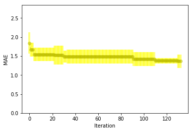
Two inches of error isn’t particularly great, but Seattle rain varies from 0 to 10 inches throughout the year, so we’re not unimpressed. Let’s see how our model improved over time by replicating a feature of the DAI UI.
# Add scores from experiment iterations
iteration_data = h2oai.list_model_iteration_data(
    initial_training_model.key
    , 0
    , len(initial_training_model.iteration_data)
)
iterations = list(map(lambda iteration: iteration.iteration, iteration_data))
scores_mean = list(map(lambda iteration: iteration.score_mean, iteration_data))
scores_sd = list(map(lambda iteration: iteration.score_sd, iteration_data))

# Add score from final ensemble
iterations = iterations + [max(iterations) + 1]
scores_mean = scores_mean + [initial_training_model.valid_score]
scores_sd = scores_sd + [initial_training_model.valid_score_sd]


plt.figure()
plt.errorbar(iterations, scores_mean, yerr=scores_sd, color = "y",
             ecolor='yellow', fmt = '--o', elinewidth = 4, alpha = 0.5)
plt.xlabel("Iteration")
plt.ylabel(initial_training_model.scorer)
plt.ylim([0, max(scores_mean) + 1])
plt.show();
Next, we’ll look at which features were most important to our model. This could include both original features and those engineered for us by DAI.
# Download Summary of Model
summary_path = h2oai.download(src_path=initial_training_model.summary_path, dest_dir=".")
dir_path = "./h2oai_experiment_summary_" + initial_training_model.key
subprocess.call(['unzip', '-o', summary_path, '-d', dir_path], shell=False)

# View Top Features
features = pd.read_table(dir_path + "/ensemble_features.txt", sep=',', skipinitialspace=True)
features.head(n = 10)
| Relative Importance | Feature | Description | |
|---|---|---|---|
| 0 | 1.00000 | 31_end_of_month~get_dayofyear | Dayofyear extracted from 'end_of_month' |
| 1 | 0.35198 | 29_TargetLag:20 | Lag of target for groups [] by 20 time periods |
| 2 | 0.34724 | 32_EWMA(0.05)(2)TargetLags:13:17:18:19:20:23:2... | EWMA (α = 0.05) of twice differentiated target... |
| 3 | 0.25388 | 31_end_of_month~get_month | Month extracted from 'end_of_month' |
| 4 | 0.16647 | 29_TargetLag:13 | Lag of target for groups [] by 13 time periods |
| 5 | 0.16609 | 35_EWMA(0.1)(2)TargetLags:rain_gauge.13:17:18:... | EWMA (α = 0.1) of twice differentiated target ... |
| 6 | 0.15684 | 32_EWMA(0.05)(1)TargetLags:13:17:18:19:20:23:2... | EWMA (α = 0.05) of differentiated target lags ... |
| 7 | 0.15396 | 29_TargetLag:17 | Lag of target for groups [] by 17 time periods |
| 8 | 0.15244 | 29_TargetLag:19 | Lag of target for groups [] by 19 time periods |
| 9 | 0.14128 | 35_EWMA(0.1)(1)TargetLags:rain_gauge.13:17:18:... | EWMA (α = 0.1) of differentiated target lags [... |
We didn’t give our AI a lot to work with, only a date and an amount of rain. Still, it was able to test out many new features.
Our top feature is the day of year, which, since we only have monthly data, is fairly similar to the 4th feature: month. Other important features include the amount of rain for various months last year and several exponetial weighted moving averages which will take into account the amount of rain for various months this year.
Retraining Our Model
Now that we have a base model that has been trained, validated, and tested we will take this model and it’s features and rebuild it on our full training data set. This will prepare us for our final goal of predicting 2016 rain per month!
# Look at model parameters
params_retrain = params
params_retrain.dump()
{'dataset_key': 'ladacasa',
 'resumed_model_key': '',
 'target_col': 'rain_inches',
 'weight_col': '',
 'fold_col': '',
 'orig_time_col': 'end_of_month',
 'time_col': 'end_of_month',
 'is_classification': False,
 'cols_to_drop': ['C1'],
 'validset_key': '',
 'testset_key': 'comobogo',
 'enable_gpus': True,
 'seed': 1234,
 'accuracy': 10,
 'time': 4,
 'interpretability': 8,
 'scorer': 'MAE',
 'time_groups_columns': ['end_of_month', 'rain_gauge'],
 'time_period_in_seconds': 2592000,
 'num_prediction_periods': 12,
 'num_gap_periods': 0,
 'is_timeseries': True,
 'config_overrides': None}
# rebuild from our previous model rather than starting over
params_retrain.resumed_model_key = initial_training_model.key

# train on the train + test dataset
params_retrain.dataset_key = retrain.key
# include no data set
params_retrain.testset_key = ''
full_training_model = h2oai.start_experiment_sync(
    **params_retrain.dump()
)
Making Predictions on New Data
Now that we have our final model we can make predictions on rain for 2016.
# Score on new data set
prediction = h2oai.make_prediction_sync(
    full_training_model.key
    , '/../../data/rain_predict.csv'
    , output_margin = False
    , pred_contribs = False
)
# Download predictions
pred_path = h2oai.download(prediction.predictions_csv_path, '.')
pred_table = pd.read_csv(pred_path)
pred_table.head()
| rain_inches | |
|---|---|
| 0 | 5.667750 |
| 1 | 2.470040 |
| 2 | 2.963274 |
| 3 | 3.453645 |
| 4 | 3.425199 |
# Join our predictions to our actauls
# Concat columns as they are in the same order
prediction_py_preds = pd.concat([predict_py.reset_index(drop=True), pred_table], axis=1)
prediction_py_preds.columns = ['rain_gauge','end_of_month','rain_inches_actual','rain_inches_prediction']
prediction_py_preds.head()
| rain_gauge | end_of_month | rain_inches_actual | rain_inches_prediction | |
|---|---|---|---|---|
| 0 | RG01 | 2016-01-31 | 8.22 | 5.667750 |
| 1 | RG01 | 2016-02-29 | 4.02 | 2.470040 |
| 2 | RG01 | 2016-03-31 | 6.05 | 2.963274 |
| 3 | RG01 | 2016-04-30 | 1.60 | 3.453645 |
| 4 | RG01 | 2016-05-31 | 1.40 | 3.425199 |
# MAE
np.absolute(prediction_py_preds['rain_inches_prediction'] - prediction_py_preds['rain_inches_actual']).mean()
2.3919339019607837
We have a 2016 MAE that’s about a 1/4 inch worse than when we tested with 2015. A couple inches of rain isn’t wonderful, let’s see what we worst at predicting.
pred_by_rg = prediction_py_preds.groupby(prediction_py_preds['rain_gauge']).apply(
    lambda x: np.absolute(x['rain_inches_prediction'] - x['rain_inches_actual']).mean())

plt.barh(pred_by_rg.index, pred_by_rg, align='center', alpha=0.5)
plt.yticks(pred_by_rg.index)
plt.title('MAE by Rain Gauge')

plt.show()
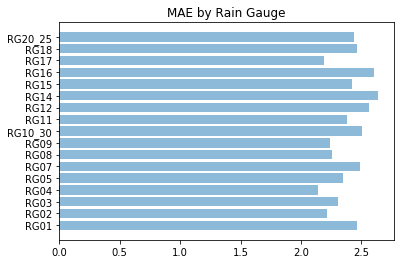
Overall, we’re fairly consistent accross the different Seattle locations. How were our predictions for different months?
pred_by_month = prediction_py_preds.groupby(prediction_py_preds['end_of_month'].dt.month).apply(
    lambda x: np.absolute(x['rain_inches_prediction'] - x['rain_inches_actual']).mean())

plt.barh(pred_by_month.index, pred_by_month, align='center', alpha=0.5)
plt.yticks(pred_by_month.index)
plt.title('MAE by Month')
ax = plt.gca()
ax.invert_yaxis()
plt.show()
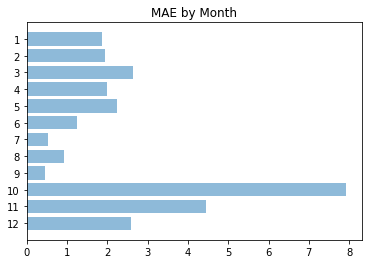
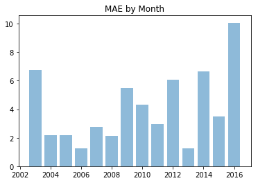
We see that our model was particularly bad for October. When we look at the overall october trends we see that the 2016 rain fall for October was 3” more that the previous rainiest October (2003) So… it’s reasonable we didn’t catch that.
october_data = rain_pivot[rain_pivot['end_of_month'].dt.month == 10]
oct_by_year = october_data.groupby(october_data['end_of_month'].dt.year).mean()

plt.bar(oct_by_year.index, oct_by_year.rain_inches, align='center', alpha=0.5)
plt.title('Amount of October Rain by Year')
plt.show()
Conclusions
Overall, in just a couple of hours we built hundereds of models (or at least we facilitated the building of 100s of models), tested many derivered features, and optimized both. Outside of the data prep, this could have been fully ran from the browser version of Driverless AI which would reduce our run time down to ~1.5 hours of us drinking coffee while our computer worked.
We all know the trope that in Seattle it’s ALWAYS raining, but we now know that Seattle is fickle about the AMOUNT of rain. With that in mind, we’re pretty happy with our results :)